Peak Finder
This Peak Finder algorithm has been designed for the detection and grouping of time-domain electromagnetic (TEM) anomalies measured along flight lines. Anomaly markers can be exported to Geoscience ANALYST, along with various metrics for characterization and targeting:
Amplitude
Dip direction
Mad Tau (TEM data only)
Anomaly skewness
While initially designed for TEM data, the same application can be used for the characterization of anomalies of mixed data types (e.g. magnetics, gravity, topography, etc.).
New user? Visit the Getting Started page.
Application
The following sections provide details on the different parameters controlling the application. Interactive widgets shown below are for demonstration purposes only.
[1]:
from geoapps.peak_finder.application import PeakFinder
app = PeakFinder(geoh5=r"../../../assets/FlinFlon.geoh5")
app()
Project Selection
Select and connect to an existing geoh5 project file containing data.
OR
Select a *.ui.json input file to re-load parameters from. See the Input ui.json section for details.
[2]:
app.project_panel
See the Project Panel page for more details.
Object/Data Selection
List of Curve objects available containing line data. Multiple data channels and/or data groups can be selected.
[3]:
app.data_panel
Flip Y-axis
Option to invert the data profile by a -1 multiplication. Useful for the detection of lows instead of highs.
[4]:
app.flip_sign
TEM data
Flag the selected data to be Time-Domain EM data.
[5]:
app.tem_box
This option enables the TEM System, Time Groups and Decay Curve panels.
TEM System
List of available TEM systems. The application will attempt to assign the Survey Type based on known channel names (e.g. Sf => VTEM).
[6]:
app.system
Assigning the right time gates to each data channel is important for the calculation of the Slanted Tau parameter.
Channel Groups
The detection and grouping of anomalies is based on property_groups, or group of channels, found on the target curve object. These groups can be defined manually by the user in Geoscience ANALYST, or auto-generated from this application.
See the Methodology section for details on how the grouping of anomalies is performed.
[7]:
app.groups_panel
Use-Create Defaults [Optional]
Create (6) pre-defined groups of data channels with corresponding default colors. Selected Data channels are assigned to three based groups (early, middle, late), with three larger overlapping groups (e.g. anomalies found in both the early and middle channel groups would be labeled as early+middle).
[8]:
app.group_auto
Decay Curve
Plot of peak values as a function of time for the nearest anomaly to the Center location.
[9]:
app.decay_figure
[9]:
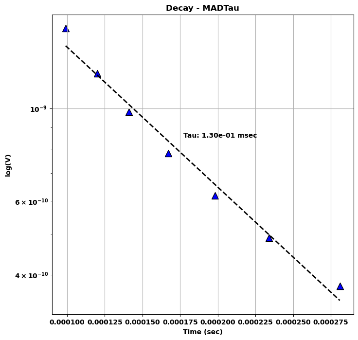
Slanted Tau
This pseudo-decay curve can be used for the calculation of the Slanted Tau, or Mad Tau, as defined by the slope of the linear fit of log( dB/dt(V)) as a function time (s).
\begin{equation} \tau = \cot(\theta) \approx \frac{\Delta t}{\Delta log(dB/dt)} \end{equation}
where \(\Delta\) denotes the varation of time \(t\) and \(dB/dt\) over the selected group of time channels (Nabighian & Macnea, 1991).
Line Selection
Selection of a channel representing the line identifier and specific line number.
[10]:
app.lines.main
The detection algorithm is applied immediately on the selected line as a test dataset. Users are invited to adjust the different Detection Parameters before Executing the process on all lines.
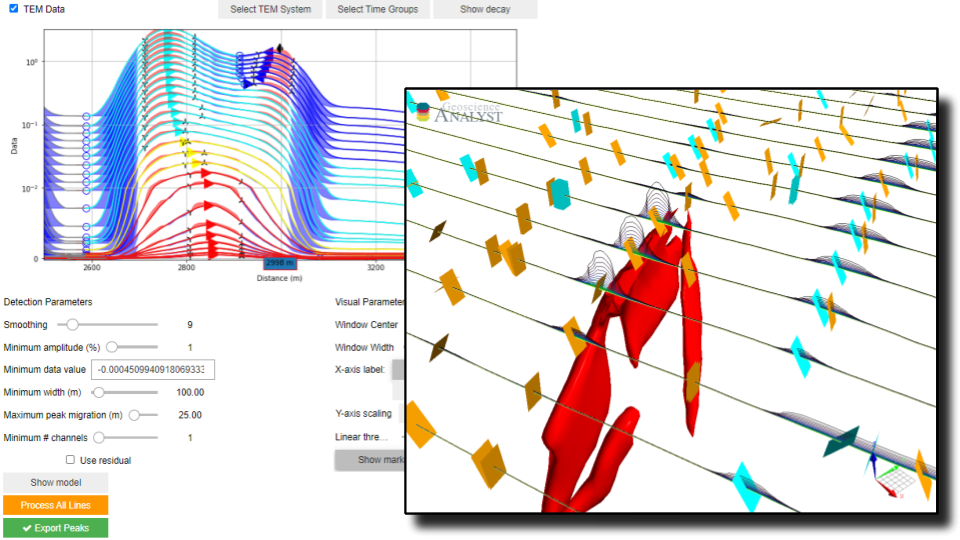
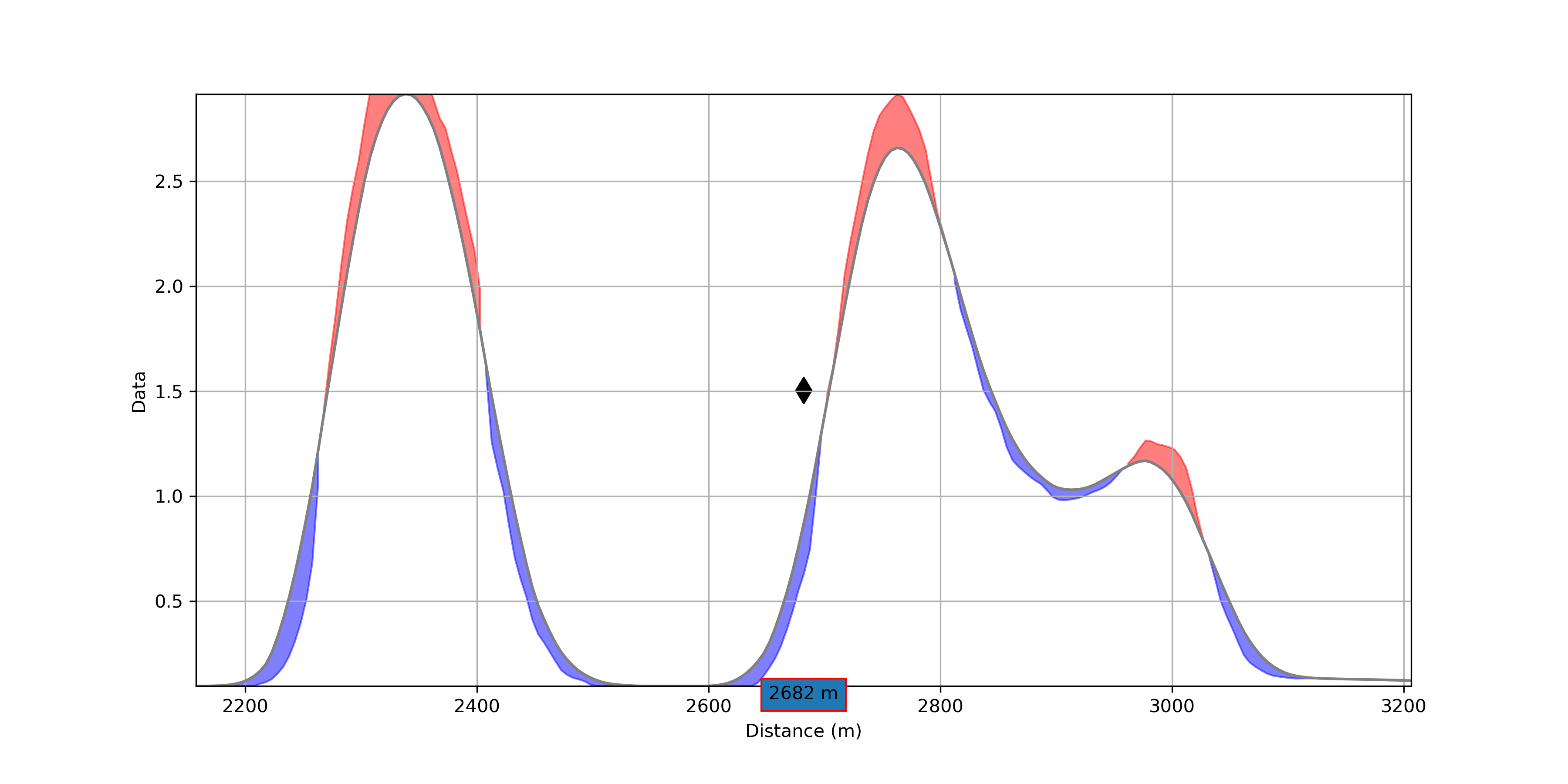
Profile Plot
Data profile plot with detected anomalies color coded by Groups.
[11]:
app.figure
[11]:
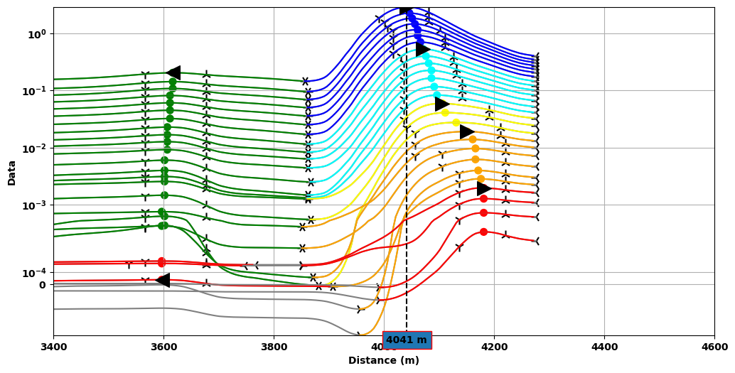
Anomalies are detected when a peak (maximum) can be found between two lows (minimum) and two inflection points. The dash line marks the position of the peak for one of the anomalies from which an estimated dip direction is determined based on:
(TEM data) the peak migration direction
(None-TEM) the skew direction
Visual Parameters
Parameters controlling the Profile Plot.
[12]:
app.visual_parameters
Select Peak
Selection of detected peaks. Used to center the plotting window and display of the decay curve.
Center
Position of the plotting window along the selected line.
Width
Width of the plotting window
X-axis label
Units displayed along the x-axis
Y-axis scaling
Normalization of the data displayed along the Y-axis
Detection Parameters
Parameters controlling the filtering and grouping of positive peak anomalies.
[13]:
app.detection_parameters
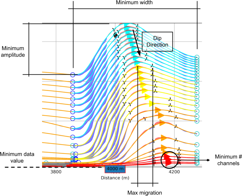
Minimum Amplitude
Threshold value (\(\delta_A\)) for filtering small anomalies:
\begin{equation} \delta_A = \|\frac{d_{max} - d_{min}}{d_{min}}\| * 100 \end{equation}
Set as a percent (%) of the data anomaly over its minimum value.
Minimum Data Value
Minimum absolute data value (\(\delta_d\)) used by the algorithm: \begin{equation} d_i = \begin{cases} d_i & \;\text{for } d_i > \delta_d \\ nan & \;\text{for } d_i \leq \delta_d\\ \end{cases} \end{equation}
Minimum Width
Minimum anomaly width (m) as measured from start to end (consecutive lows).
Maximum Peak Migration
Threshold applied on the grouping of anomalies based on the lateral shift of peaks.
Smoothing
Parameter controlling the running mean averaging:
\(d_i = \frac{1}{N}\sum_{j=-\frac{N}{2}}^{\frac{N}{2}}d_{i+j}\)
where N is the number of along line neighbours used for the averaging. The averaging becomes one sided at both ends of the profile.
Show residual
Option to show the positive (blue) and negative (red) residuals between the original and smoothed profile. Useful to highlight smaller anomalies within larger trends.
Output Panel
Run and export anomaly markers.
[14]:
app.output_panel
Process All
Run the search algorithm on all lines. This process is run in parallel using Dask. Anomaly group markers are exported to the target geoh5 project.
All Markers
Write the full set of markers (min, max, inflections) for all peaks on every data channels.
See the Output Panel page for more details.
Methodology
This section provides technical details regarding the algorithm used for the detection of 1D anomalies.
Anomalies are identified from the detection of maximum, minimum and inflection points calculated from the first and second order derivatives of individual data channels. The algorithm relies on the Numpy.fft routine for the calculation of derivatives in the Fourier domain.
Detection Parameters are available for filtering and grouping co-located anomalies. The selection process is done in the following order:
Primary detection
Loop over the selected data channels:
Apply the Minimum Data Value threshold.
For every maximum (peak) found on a profile, look on either side for inflection and minimum points. This forms an anomaly.
Keep all anomalies larger than the Minimum Amplitude
Grouping
Anomalies found along individual data channels are grouped based on spatial proximity:
Find all peaks within the Maximum Peak Migration distance. The nearest peak is used if multiple peaks are found on a single channel.
Create an anomaly group that satisfies the following criteria:
The data channels must be part of a continuous series (maximum of one channel skip is allowed)
A group must satisfy the Minimum number of channels
For TEM data, an ID gets assigned based on the largest overlap between the labeled data channels and the pre-defined Channel Groups.
Input ui.json
This application relies on a structured json file to store and run the program.
The same input ui.json file can be used to run the program from command line:
activate geoapps
python -m geoapps.peak_finder.driver [input].ui.json
or directly from Geoscience ANALYST Pro v3.3.1 or higher. The ui.json can also be used to re-load the parameters from a previous run by selecting the ui.json file from the Project Selection widget, instead of a geoh5 file.
Notes
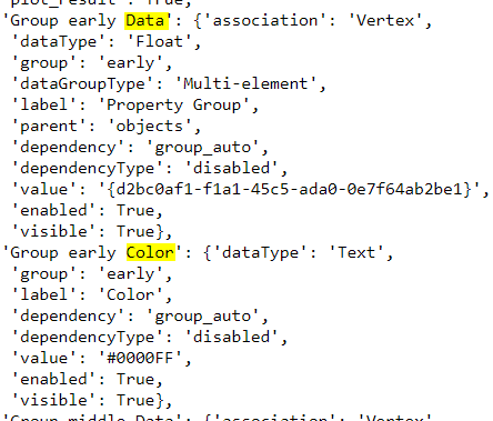
Additional groups can be used by adding new blocks of parameters to the default input ui.json file:
For each additional group blocks, a unique name must be provided (C, D, etc)
Changes made will be displayed after re-loading the ui.json from the Project Selection panel.
Geoscience ANALYST Pro v3.4
Users with an active Geoscience ANALYST Pro license (v3.4) can execute this application directly from an active session with a drag & drop of a *.ui.jsonfile to the Viewport.
Need help? Contact us at support@mirageoscience.com